2026-04-16

Some Learnings from TurboQuant

This post is made without AI assistance, so do pardon my grammar.

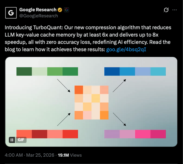
Tldr; We are trying to reduce the amount of space LLM take RAM wise as token amount grows. How we do this can be achieve through TurboQuant, which is a combination of PolarQuant and QJL, and it aims to prevent bottleneck by RAM by reducing the size of KV cache, but it the place of the reduced space, more calculation needs to be done, but at increasing context, the trade-off moves towards a net positive.

How the average flow of a attention level looks like is something like this:

Input -> Operation (read from KV cache (1 to ...n-1th term) -> write to KV cache nth term) -> output.

The contribution/ changes mostly lie on the write step, and read can be understood as a reverse of it.

Post TurboQuant, the WRITE and READ step looks something like this.

WRITE (every new token):
	compute k
	-> rotate (multiply with orthogonal matrix)
	-> polar convert -> arctan recursion -> one radius(norm) + angles
	-> Lloyd-Max quantization (optimal for gausian)
	-> compute sign bits of error (rotated K - quantized K)
	-> store: indicies + FP32 norm + sign bits of error. 
	
READ (every query)
	fresh Q arrives 
	-> reconstruct approximate K (reverse polar (convert to cartesian, x norm)
	-> compute Q · reconstructed K (new K vector)
	-> compute Q · sign(ε) (bias correction)
	-> add together -> unbiased attention score 
	-> softmax across all cache region -> weights
	-> weighted sum of compressed V -> output.

Essentially we're changing storing the whole KV cache in it's entirety, which can go up to 40GB of ram on a llama3 70B as it approaches 128k token context, and breaking it up into several pieces and construct it when needed. This involves rotating, convert to polar coords, Lloyd-max quantization, compute sign bits, all done on the K tensors pre- any transformation, so raw values essentially. Then at read time, angles are de-quantized via lookup and scaled by the norm to reconstruct an approximate K vector, and we'll use the sign bits saved to nudge it back, make more accurate to pre-quantize. The mathematical basis is that after rotation then coordinates follow a known gaussian distribution of limit (constructed from arctan [-pi, pi]) which means Lloyd-Max buckets boundaries can be pre-computed once and reused forever, eliminating the per-block overhead (conventional way is storing min-max to reverse, this avoids that).

For reference, storage looks something like this:

K: indicies + norm + sign bits (PolarQuant + QJL)
V: indicies + norm             (PolarQuant)

Been a few months since I graduated, have some time in-between job search, and my recent obsession is on AI optimization, specifically the math side of it, so decided to give the paper TurboQuant a go. If you've been keeping up with tech news, TurboQuant should't sound unfamiliar to you, its a paper released by Google on reducing the RAM bottleneck of Large Language Models, when the news broke, memory stocks like MU, WDC, and SDK all dropped. So we'll be going a bit over what TurboQuant specifically is, and it's implications.

I'll be writing this in the way on how I learned it, I'll also include some "why?" part to make it make sense in first principles why certain things are included, hopefully this is able to help you develop intuition on the architecture.

The first story of the day would be TurboQuant. Its an paper released by Google to reduce KV cache in Large Language Models (I.e., Models are more efficient, less compute is required for same amount of reasoning).

Understanding why KV Cache is a problem?

For specifics on what KV cache is, you can refer to my past paper on Transformer and So On. But for a quick recap, in autoregressive model, attention need to compute the KV Cache to decide the logits and find the most suitable next token, and is represented as such.

\text{Attention}(Q, K, V) = \text{softmax}(QK^{T} / \sqrt{d}) \cdot V

Since to predict the next token with proper context, we use all previous KV vectors (i.e., cumulative from 1st to n-1 th token), and instead of recalculating the KV cache with each token, we simply cache them, but that leads us to another bottleneck, especially when context grows. A single 128k-token prompt on Llama 3 70B consumes roughly 40GB of high-bandwith memory on datacenter GPUs, or unified memory on apple silicon just for caching. Cache grow can be calculated with $O(n \cdot L \cdot d)$ , where its sequence length x layers x head dimension, all in fp16, and as context length grows, you'll spend more time transporting KV vectors from memory to compute cores than actually doing the matrix multiplications. Here's where TurboQuant comes in, it essentially compresses the amount of data (3~4x ) that you need to transport across the bus per attention step.

With that you can sort of see why this might be a problem to the direction that the industry wants to go in with the whole agentic narrative. It becomes quite expensive for models to work on actual task, especially with the RAM shortage, and the typical agentic task, typically involves multiple tool calls, long reasoning chains, past contexts, all inflates the context easily past 100k+ tokens, thus making this paper that much important.

What do we do?

Essentially, instead of storing the KV cache in its entirety original form, we break it down like how we transport furniture, into parts that takes up less space in storage and only constructed when use. So how does this work technically? It can be broken into 2 parts, which stems from 2 previous papers, PolarQuant and QJL.

We first start with Polar Quant.
The goal is here random rotation + arctan polar transformation + scalar quantization. Now why would we wanna do that? Remember we're trying to reduce the space of the KV cache and to ensure that we have as little "whitespace" as possible, we use polarQuant to ensure the numbers are as "tight" as possible. What it does is it first rotate the matrix, we rotate it with a orthogonal matrix (recall matrix is orthogonal if $X^{T}X = I$ ), and ensure the energy is spread across all matrix, so outliers wouldn't cause all value to be to be squeezed into some concentrated quadrant/ bin when we move to quantization step. Now, after the rotation, the distribution would be gaussian in nature.

In mathematical notation, the rotation looks something like this:

We take a vector $x \in \mathbb{R}^{d}$ . Apply a random orthogonal matrix R (a Hadamard or random Gaussian rotation) $\tilde{X} = Rx$ Now, since the R is orthogonal, $||\tilde{X}|| = ||X||$ , the norm (radius/ size) is preserved exactly, while the energy is now spread uniformly across all coordinate. To visualize, I'll provide an example in numbers (varience is lower is what we want):

[0.02, 0.01, 7.8, 0.03, -6.9, 0.01, 0.02, 5.4] -> [1.1, -0.9, 1.3, -1.0, 0.8, -1.2, 1.1, -0.9]

After the rotation, just before we quantize them, we want to transform them into polar coordinates. Why? this is to reduce the overhead when storing the values, and when we want to reverse the values back during read (We'll go into more detail later). How we polar transform is we convert the coordinate from cartesian based to polar based recursively, pairing up coordinates and using arctan to extract an angle and radius, then taking the resulting radius and pairing it with the next coordinate,

(\tilde{x}_1, \tilde{x}_{2}) \\

Convert to polar:

r = \sqrt{({\tilde{x}_{1}}^{2} + {\tilde{x}_{2}}^{2})} \quad ← \text{radius}

\theta = \arctan(\tilde{x}_{2} / \tilde{x}_{1}) \quad ← \text{angle (the "degree" part)}

The arctan is where the angle come from. Then you recurse, take that r, pair with the next coordinate x̃₃, convert again: $(r, \tilde{x}_{3}) → (r_{2}, \theta_{2})$ repeat this until we have one final radius (norm) and $d-1$ angles.

This step is what allows Lloyd-Max quantization (next step) to work without per-block overhead, the angles follow a known fixed distribution (the coords are gaussian, and the arctan of gaussian-distributed pairs, follows a well, fixed distribution of -pi, pi) after rotation, so quantization boundaries are pre-computed once and reused forever. Only the final radius needs to be stored as bookkeeping, in full precision, FP32.

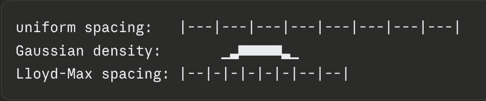
Since the coordinate now follows a known distribution. We can proceed to the quantization to reduce the size, in this case, since the distribution is known to be gaussian, we can go ahead an use the the optimal method, Lloyd-Max quantization, it minimizes quantization errors by placing quantization levels at the centroid of a gaussian instead of uniformly spaced (Its preferred over the uniformly choice, as in a gaussian distribution, data tends to be concentrated around some numbers, like 0, and if we use a uniform spacing, it'll have the problem where a handful of bins have high concentration, where the majority of others don't, reducing quality). Thus, Lloyd-Max is optimal among scalar quantizers for this distribution, and the full TurboQuant scheme approaches the Shannon-rate distortion bound.

Looks something like this:

LLoyd Max vs fixed size quantization comparison

Storing the norm: The only overhead we're storing is $||X||$ (the vector norm), once per vector as a single float. This is 4 bytes per 128-dimensional vector vs 256 bytes (128 x FP16), a tiny fraction. Traditional vector quantization usually introduces its own memory overhead, as most methods require calculating and storing quantization constants for every small block of data, adding 1 or 2 extra (min max) bits per number; but TurboQuant avoids this by operating on the whole-vector level.

So what's in storage now is:

128 quantized angles x 3 bits each = 48 bytes 
+ 1 norm in FP32                   = 4 bytes 
total                              = 52 bytes  (PolarQuant only)

Next we move on to QJL (Quantized Johnson-Lindenstrauss). After PolarQuant Compresses K, a small error remains, the gap between where the actual K position was, and where the nearest quantization bucket landed. This would be $\epsilon = x_{\text{rotated}} - x_{\text{quantized}}$ , based on the rotated coordinate space. Now, instead of storing all these error in cache, (which we don't need to btw), we just store the sign's themselves. In computing attention, we only ever need <Q, K>, the inner product, and not K itself.

So to maintain the precision, intuitively, you'd think we need the whole error, but no, you really just need an accurate dot product. What does this mean? We simply need the sign itself (+, -). For each coordinate of $\epsilon$ , we store a +1, or a -1, a bit per coordinate.

So storage now looks something like this:

128 quantized angles x 3 bits each = 48 bytes (PolarQuant)
+ 1 norm in FP32                   = 4 bytes  (PolarQuant)
--- 
+ 128 sign bits x 1 bit each       = 16 bytes (QJL)
total                              = 68 bytes

as compared to traditional method of where it stores 128 bit x 16 bits each at FP16, which becomes 256 byte. Approx, a ~3.5-3.7x reduction in space consumed, depending on head dimension.

Now, thats writing to KV cache, how about during read time?
We are, loosely speaking, trying to reverse what we've done (To be more precise, we don't really full reverse the polar recursion transformation, but more, de-quantize the angle indicies directly back to approximate Cartesian coordinates via lookup, then scale the norm).

So as a fresh full-precision Q arrives:

we reconstruct the approximate K through reversing the polar coords to cartesian based, and multiply it by the norm,
we compute the Q $\cdot$ approximate K for a new K vector,
then we take the Q and multiply it with the sign bits ( $\epsilon$ ) to remove the bias,
add them (step 2 & 3) together for an unbiased attention score,
typical transformer attention. we softmax over all cache attention score,
we compute the weighted sum of the compressed V vectors and have a final output.

Some final thoughts,

one thing I don't see discussed enough (afaik), is enterprise adopting and boasting (some) cloud AI don't seemed to recognize the fact that they're trading productivity gains for long-term leverage. Model providers have a track record of internalizing whatever generates the highest return from the ecosystem and building on top of them, and you can kinda see, at some point it simply is more financially rewarding for them to replace whole operations as opposed to the subscription fee they provide. Now, I'm not saying local inference is the solve-all to this problem, but it's a direction I think is quite low-friction and worth exploring more, and tools like TurboQuant, even though aimed probably to make Google's TPU more efficient, inevitably does benefit everyone that tries to deploy them, making self-hosting more than just a toy.

Anyways, that's the end of it, if you made it this far, thanks for reading.

Footnotes:

Shannon Rate-Distortion: What is the minimum number of bits fundamentally needed to represent a source at some given level of distortion. For a gaussian source, the following is the answer. $R(D) = \frac{1}{2} \log_{2}(\sigma^{2} / D)$ How to read? If the source has some variance of $\sigma^{2}$ , and you're willing to tolerate distortion of D, you'll need at least R(D)bits, that's the physical limit, no scheme in existence can do it in fewer. Intuition: As $\sigma^2$ increases, the range of value becomes bigger, more "surprising", harder to predict, requiring more bits to describe. As D increase, you're tolerating more distorted levels, less bits, increasing the sloppiness of the representation.
Memory Structure: Every thing stored in a computer comprises of just a patters of bits. The question is how much bits you dedicate to each number.

Post PolarQuant, the data looks something like this:

128 quantized angles x 3 bits each = 48 bytes 
+ 1 norm in FP32                   = 4 bytes 
total                              = 52 bytes

Instead of storing the whole data in 16 bits per coordinate, we store them in 3 bits per coordinate and the norm in one single FP32 digit. Making storage be 256 bytes -> 52 bytes, around a 5x improvement for PolarQuant alone, and ~3.7x improvement for the full TurboQuant scheme including QJL sign bits.

For reference:

FP32  = 32 bits = 4 bytes per number (High Precision)
FP16  = 16 bits = 2 bytes per number (Half Precsion)
INT8  = 8 bits  = 1 byte  per number (Low Precision)
3-bit = 3 bits  =         per number (very low precision)

How does this look in inference time?

(1.) take the quantized angles then 
(2.) dequantize angle indices via lookup and 
(3.) reconstruct approximate k vector scaled by the stored norm.

V Storage and Process: V is only processed with PolarQuant, as compared to K, which means no sign bits are stored, this is because V is used in weighted sum, not a dot product with Q, so there is no systematic bias to correct. The following is the steps for a bit of visual reference:

scores = Q · Kᵀ           ← dot product, giving raw scores per token
weights = softmax(scores) ← converts scores to probabilities scalars
output = weights · V      ← each V vector scaled by its scalar                                  weight, then summed.